A brief tutorial

Installation

To install aldenv use:

pip install aldenv

ALD models

aldenv implements a series of surface kinetic models based on irreversible first order Langmuir kinetics. The four models currently implemented are:

• SingleALD: ALD model with a single reaction pathway
• MultiALD: ALD model with multiple reaction pathways
• SoftSatALD: a specific case of MultiALD where the precursor has a second reaction pathway, so that it is soft-saturating.
• SingleALDCVD: ALD model with an additional CVD component characterized by the presence of a non-zero co-reactant partial pressure during the precursor dose.

All these models compute the steady state growth per cycle for a pair of dose and a precursor dose times, assuming that these are ideally separated by purge times.

For instance, we can import and define a SoftSatALD process as follows:

from aldenv.models import SoftSatALD
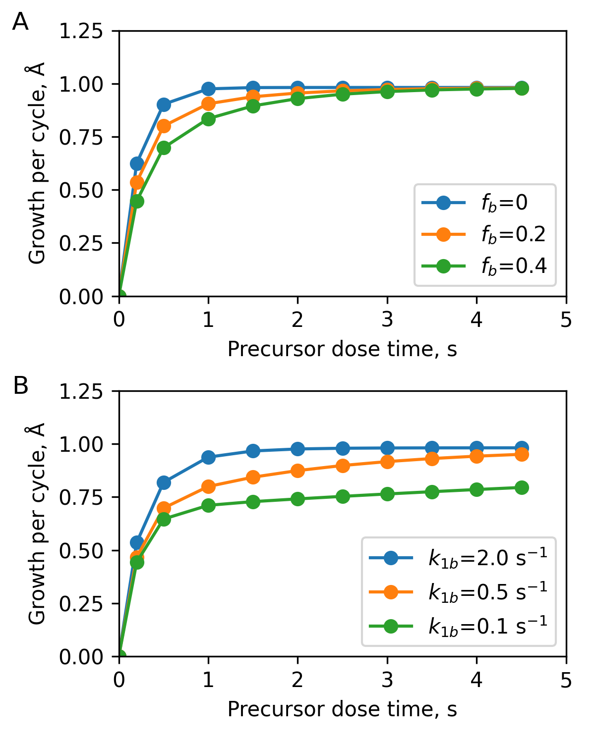
ald = SoftSatALD(k1=5, k1b=1, fb=0.2, k2=4, gpc=1)

Here, the k inputs represent the rate constants (in s^-1) and fb is the fraction of the surface sites with the rate constant k1b. The indices 1 and 2 represent the precursor and a coreactant.

The expression:

g = ald(1.0,1.0)

Here is a plot generated using SoftSatALD showing saturation curves for different parameter values:

ALD process

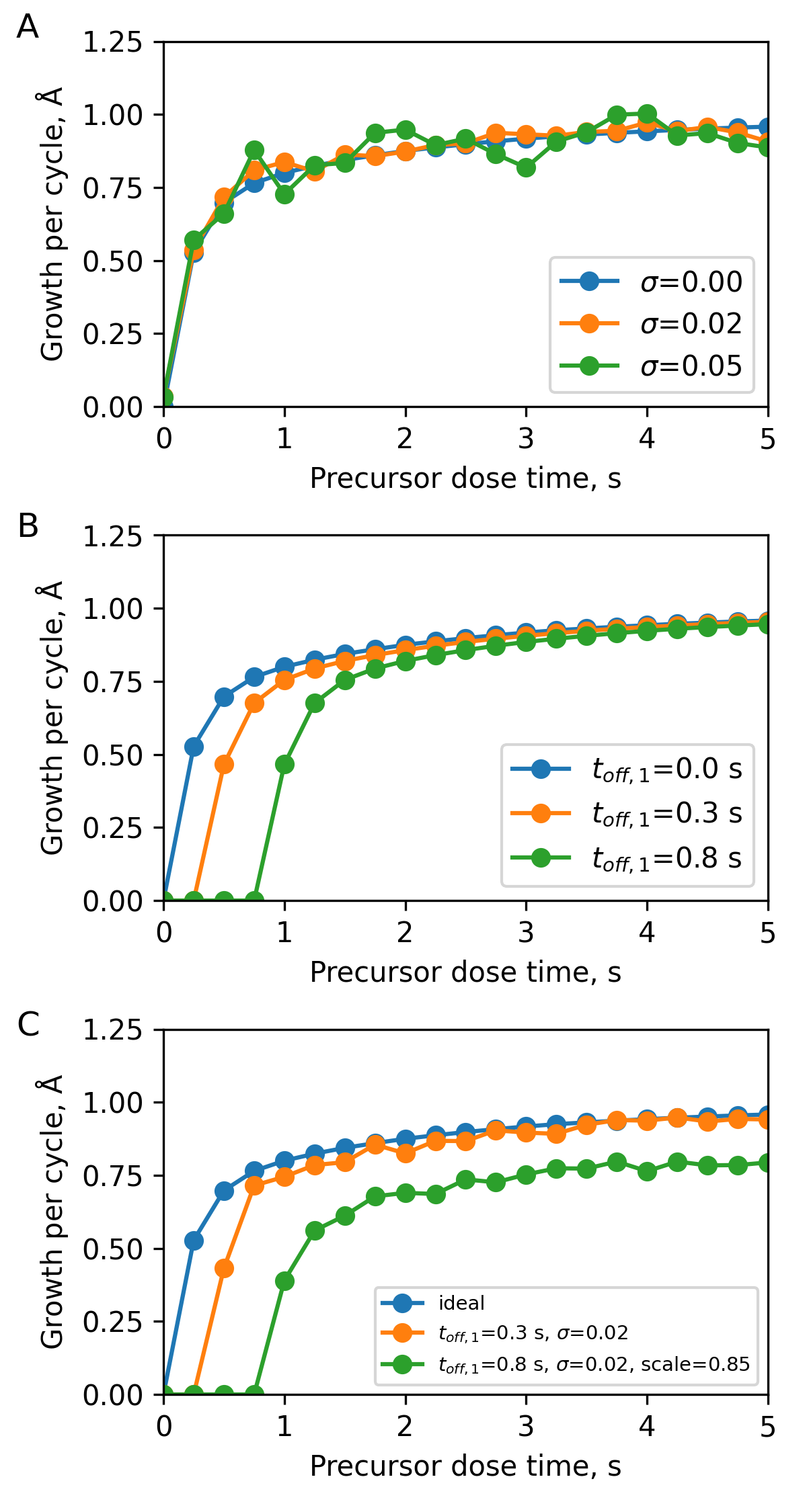
The difference between an ALD model and an ALD process, is that an ALD process incorporates some of the non-idealities that you would expect in an experimental system. These are mainly three:

• Measurement noise, added to a model's output
• Dose offsets due to upstream consumption
• Scaling factors coming from the nature of the measurement carried out to determine the growth per cycle.

The way aldenv implements this is through the use of the ALDProcess class. For instance, taking the SoftSatALD model considered above, we can implement a process as follows:

from aldenv.models import SoftSatALD
ald = SoftSatALD(5, 0.5, 0.3, 4, gpc=1)

process = ALDProcess(ald, round_to=3, toff1=0.8, noise=0.02, scale=0.85)

This implement an ALD process where the output is rounded to three significant digits, has an upstream consumption for the precursor equal to 0.8 seconds, adds a noise of 0.02, and introduces a scaling factor for the growth per cycle of 0.85.

Environments

Finally, aldenv implements a number of environments that can be used to benchmark optimization algorithms. These are meant to represent a set of generic ALD processes.

For instance:

from aldenv.envs.steadystate import FastFast

ald = FastFast(round_to=3, noise=0.01)

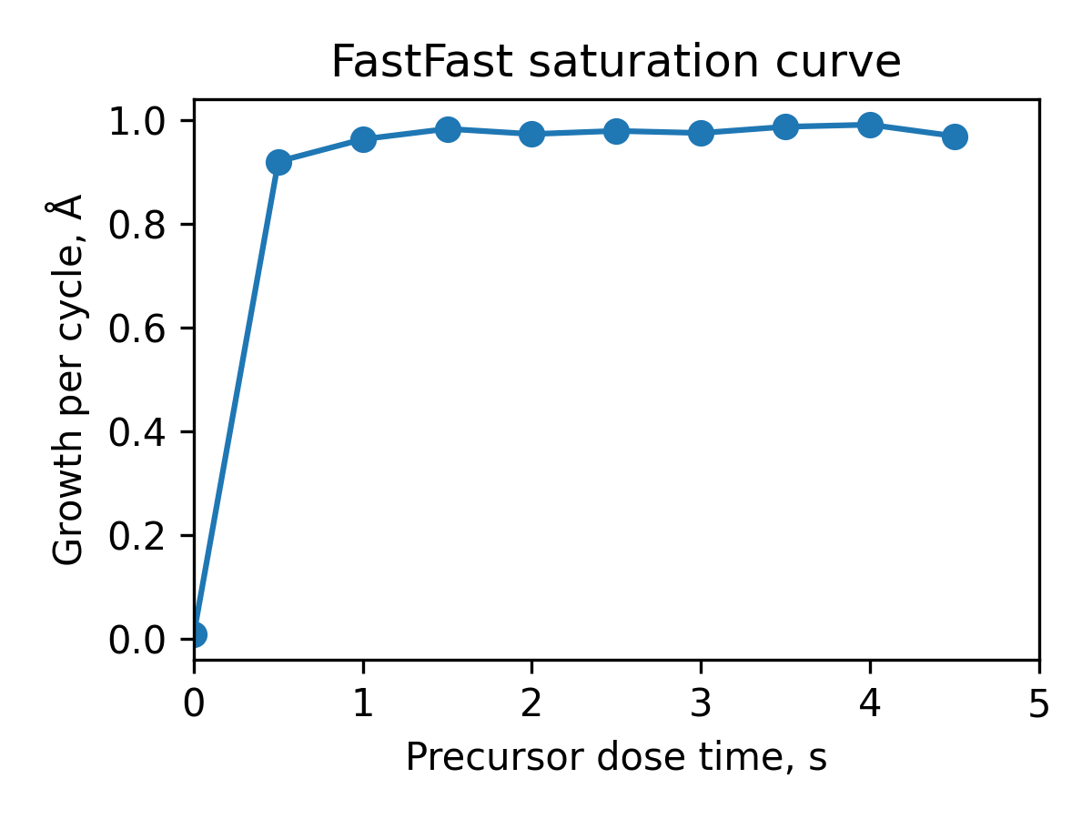
creates a fast-fast ALD process where both the precursor and co-reactant are saturated after 0.2s doses and with a saturation growth per cycle of 1 Angstrom. It considers a noise level of 0.01 Angstrom and that the output is limited to three significant digits.

Sweeping the precursor dose time gives the following saturation curve:

steadystate environments

steadystate environments contain a series of virtual ALD processes where the growth per cycle is computed as a function of the precursor and the co-reactant dose times. For instance, in our work Performance of AI agents based on reasoning language models on ALD process optimization tasks, we use the following environments included in steadystate to evaluate the ability of agents based on reasoning LLMs to optimize ALD processes:

• FastFast represents an ideal ALD process with fast saturation for both precursor and co-reactant.
• SlowFast represents an ideal ALD process where the precursor requires longer doses to saturate.
• SlowSlow represents an ideal ALD process where the precursor and the coreactant are slow to saturate.
• SoftFast introduces a soft-saturating precursor, where after a fast rise it slowly saturates.
• FastFast3 is a version of FastFast where the saturated growth per cycle is 0.3 Angstrom.

In addition to these environments, which are fully self-limited, aldenv also contains environments where the growth has a CVD component. For instance:

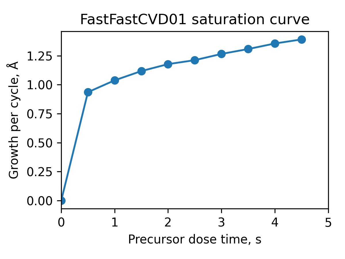
• FastFastCVD01 has a built in CVD component of 0.1 Angstrom per second. This means that a 10 second dose give you an additional Angstrom due to the non self-limited behavior.

This results in the following saturation curve:

Upstream consumption

All steadystate environments derive from ALDProcess, which wraps an ALD model and applies experimental limitations on top of its raw output.

In order to model upstream consumption, ALDProcess and all its subclasses can receive two parameters, toff1 and toff2, to create offsets. The corresponding saturation curves are computed at the effective dose times t1 - toff1 and t2 - toff2. A dose shorter than its offset is fully consumed upstream: nothing reaches the sample and the growth per cycle is 0. The defaults are toff1 = toff2 = 0, in which case there is no upstream consumption and the dose times are passed through unchanged.

For example, giving FastFast a precursor offset of 0.5 s:

from aldenv.envs.steadystate import FastFast
import matplotlib.pyplot as pt
import numpy as np

process = FastFast(round_to=3, noise=0.01, toff1=0.5)

t1 = np.arange(0, 5, 0.5)
t2 = 1.0

gpc = np.array([process(t, t2) for t in t1])

pt.figure(figsize=(4,3))
pt.plot(t1, gpc, 'o', linestyle="-")
pt.xlabel("Precursor dose time, s")
pt.ylabel(r"Growth per cycle, $\mathrm{\AA}$")
pt.title("FastFast, toff1 = 0.5 s")
pt.xlim(0, 5)
pt.tight_layout()
pt.savefig("fastfast_toff_sat.png", dpi=300)
pt.show()

produces the saturation curve below:

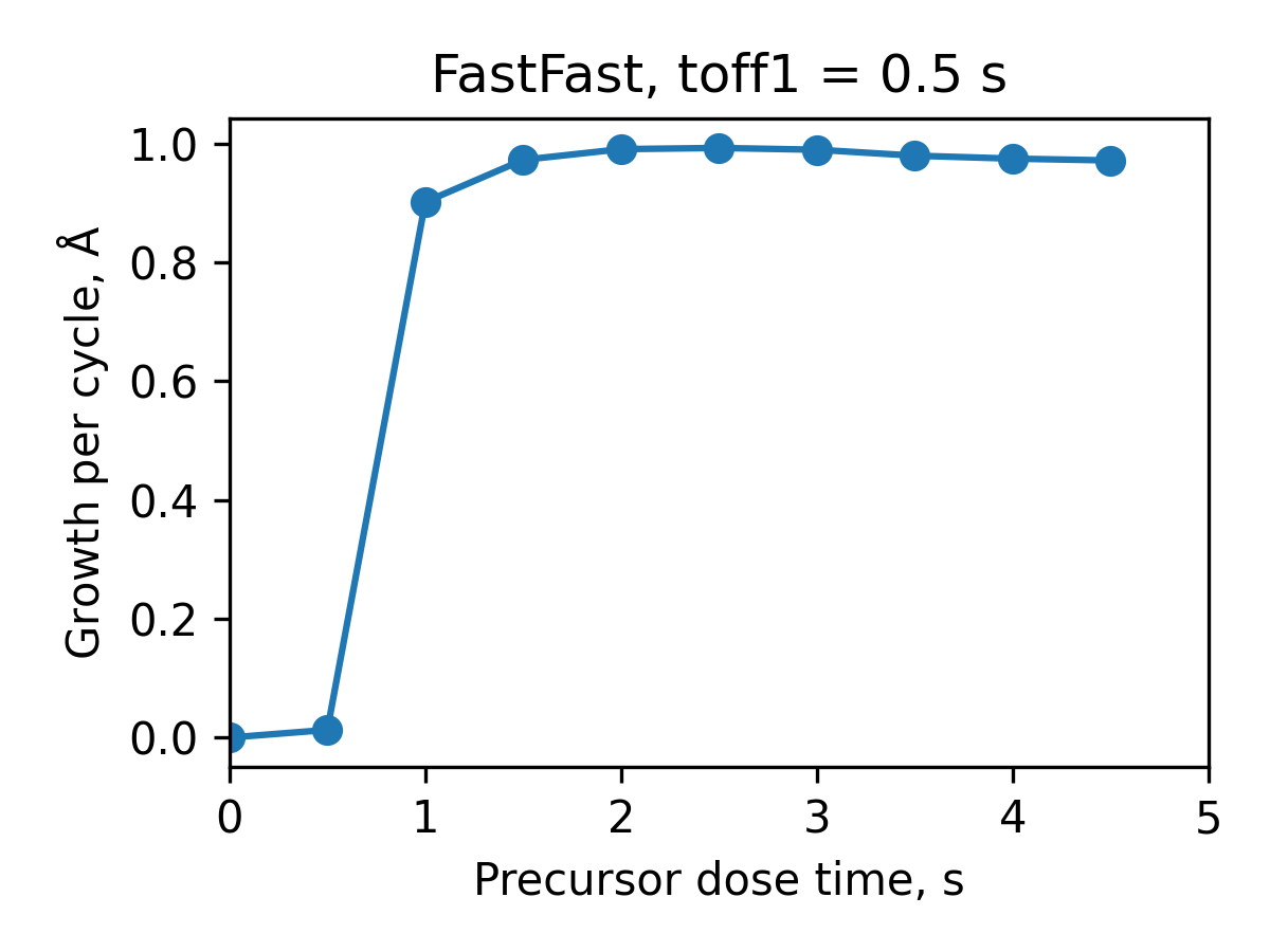
Compared with the offset-free curve at the top of this tutorial, the whole saturation curve is displaced by 0.5 s: doses of 0.5 s or shorter give no growth at all, and saturation is only reached after about 0.7 s instead of about 0.2 s. The saturated growth per cycle is unchanged.